There are three methods to compute the derivative of a function on a computer. Namely, numerical, symbolic, and automatic differentiation. Numerical differentiation uses finite-difference approximations, which are simple to implement but can be highly inaccurate due to truncation and round-off errors, and it scales poorly when computing gradients with respect to millions of parameters. Symbolic differentiation addresses these weaknesses at the cost of constructing new mathematical expressions that can, in the worst case, grow exponentially—a phenomenon known as expression swell—leading to high memory consumption. In contrast, automatic differentiation, or just autodiff, decomposes a function into elementary operations with known derivatives and uses them to propagate numerical derivative values through the computation.
Now, consider a differentiable function with input and output . The exact derivative of at is its Jacobian:
Each differentiation method computes the Jacobian differently by treating the function differently. Intuitively, numerical differentiation perturbs the inputs, symbolic differentiation rewrites the mathematical expression, and automatic differentiation propagates derivative values through elementary operations.
Numerical differentiation treats as a black box and approximates the Jacobian by perturbing one input by a small non-zero step and observing how the output changes:
Here, is the unit vector that selects . Computing the complete Jacobian therefore requires repeating this process for all inputs, in addition to the baseline evaluation of .
Symbolic differentiation treats as a mathematical expression and constructs a new expression for each derivative in the Jacobian:
The resulting matrix is therefore an exact symbolic function of , but its expressions can grow significantly.
Automatic differentiation (AD) represents the evaluation of as a computation graph of elementary operations that describes how the input values are transformed to the output . Suppose an operation in the graph computes from the values on which it directly depends. We write when directly depends on . The local Jacobian associated with this dependency is
Associating each direct dependency in the computational graph with its local Jacobian produces a linearized computation graph (LCG) that describes how small changes in the input propagate to the output.
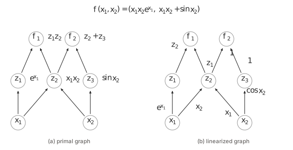
An instance of with . (a) the primal graph, whose vertices are the intermediate values and whose edges run towards the outputs; (b) the linearized graph, the same shape with every edge carrying its local Jacobian . The shared product feeds both outputs, so the graph is a diamond rather than a tree. Structure after an example of Paul D. Hovland.
For a particular evaluation of , the executed elementary operations can be represented as a directed acyclic graph (DAG). Its nodes can therefore be processed in topological order, from the input nodes () to the output nodes (), or in reverse topological order, from the outputs to the inputs.
Processing the LCG from inputs to outputs is called forward-mode. Given an input direction , forward mode initializes the input change as and applies the chain rule at every operation:
After the graph has been processed, the resulting output change is the Jacobian-vector product (JVP):
Choosing , where is the -th standard basis vector, produces
which is the -th column of the Jacobian. Therefore, the complete Jacobian can be computed using forward-mode passes (for ), and this mode is preferable when the function has considerably fewer inputs than outputs ().
Processing the LCG from outputs to inputs is called reverse-mode. Reverse mode first evaluates , and then processes this recorded computation in reverse topological order.
Given an output direction , reverse mode computes the derivative of the scalar function . For the output node , reverse mode initializes
where denotes the reverse-mode adjoint associated with . It then applies the chain rule at every node in the graph:
After the graph has been processed, the resulting input adjoint is the vector-Jacobian product (VJP):
Choosing produces
which is the -th row of the Jacobian. Similarly, the complete Jacobian can be computed using reverse-mode passes, and is preferable when the function has considerably more inputs than outputs ().
Backpropagation
A special case of reverse-mode AD, called backpropagation, is when the function has scalar output (). In this case there is only one output direction, , so the vector-Jacobian product
is the Jacobian of .
Implementation
Now, we will create a tiny library that does symbolic, numerical and automatic differentiation. For each method, we will differentiate the same function:
def f(x1, x2):
    z1 = x1 * x2 + Expr.relu(x1 - x2)
    return z1**2, x1 + 10 / z1
Note that is not differentiable at every point, which makes this example more interesting.
Symbolic differentiation
Symbolic differentiation overloads operators so that every expression constructs an immutable expression tree. Differentiation is therefore done by recursively applying a rule associated with each node.
class Expr:
    def __init__(self, op, *args):
        self.op, self.args = op, args

    def diff(self, x):
        """Return the symbolic derivative with respect to x."""
        match self.op, self.args:
            case "symbol", (name,):
                return int(name == x.args[0])
            case "+", (a, b):
                return Expr._diff(a, x) + Expr._diff(b, x)
            case "*", (a, b):
                return Expr._diff(a, x) * b + a * Expr._diff(b, x)
            case "**", (a, n):
                return n * a ** (n - 1) * Expr._diff(a, x)
            case "relu", (a,):
                # H is the Heaviside step function.
                return Expr("H", a) * Expr._diff(a, x)

    @staticmethod
    def _diff(a, x):
        """Treat ordinary numbers as constants."""
        return a.diff(x) if isinstance(a, Expr) else 0

    def eval(self, values):
        """Evaluate the expression using the supplied symbol values."""
        match self.op, self.args:
            case "symbol", (name,):
                return values[name]
            case "+", (a, b):
                return Expr._eval(a, values) + Expr._eval(b, values)
            case "*", (a, b):
                return Expr._eval(a, values) * Expr._eval(b, values)
            case "**", (a, n):
                return Expr._eval(a, values) ** n
            case "relu", (a,):
                return max(0, Expr._eval(a, values))
            case "H", (a,):
                # We define H(0) = 0 although ReLU is not differentiable at
                # zero, matching the convention.
                return int(Expr._eval(a, values) > 0)

    @staticmethod
    def _eval(a, values):
        """Leave ordinary numbers unchanged during evaluation."""
        return a.eval(values) if isinstance(a, Expr) else a

    @staticmethod
    def relu(x):
        """Apply ReLU to a symbolic expression or number."""
        return Expr("relu", x) if isinstance(x, Expr) else max(0, x)

    def __add__(self, other): return Expr("+", self, other)
    __radd__ = __add__

    def __mul__(self, other): return Expr("*", self, other)
    __rmul__ = __mul__

    def __neg__(self): return Expr("*", -1, self)
    def __sub__(self, other): return self + -other
    def __rsub__(self, other): return other + -self
    def __pow__(self, n): return Expr("**", self, n)
    def __truediv__(self, other): return self * other**-1
    def __rtruediv__(self, other): return other * self**-1

    def __str__(self):
        """Return a readable mathematical representation."""
        match self.op, self.args:
            case "symbol", (name,):
                return str(name)
            case ("relu" | "H"), (a,):
                return f"{self.op}({a})"
            case op, (a, b):
                return f"({a} {op} {b})"

    __repr__ = __str__
With this simple Expr library we can now compute the Jacobian of :
x = (
    Expr("symbol", "x_1"),
    Expr("symbol", "x_2"),
)

fx = f(*x)

J = [
    [f_i.diff(x_j) for x_j in x]
    for f_i in fx
]

def J_f(*values):
    variables = dict(zip((x_i.args[0] for x_i in x), values))

    return [
        [Expr._eval(entry, variables) for entry in row] for row in J
    ]

print("f(x) =", fx)
# ((((x_1 * x_2) + relu((x_1 + (-1 * x_2)))) ** 2), (x_1 + ((((x_1 * x_2) + relu((x_1 + (-1 * x_2)))) ** -1) * 10)))

print("f(1, 2) =", f(1, 2))
# (4, 6.0)

print("J_f(x) =", J)
# [[(((((x_1 * x_2) + relu((x_1 + (-1 * x_2)))) ** 1) * 2) * (((x_2 * 1) + (x_1 * 0)) + (H((x_1 + (-1 * x_2))) * (((x_2 * 0) + 0) + 1)))), (((((x_1 * x_2) + relu((x_1 + (-1 * x_2)))) ** 1) * 2) * (((x_2 * 0) + (x_1 * 1)) + (H((x_1 + (-1 * x_2))) * (((x_2 * 0) + -1) + 0))))], [((((((((x_1 * x_2) + relu((x_1 + (-1 * x_2)))) ** -2) * -1) * (((x_2 * 1) + (x_1 * 0)) + (H((x_1 + (-1 * x_2))) * (((x_2 * 0) + 0) + 1)))) * 10) + ((((x_1 * x_2) + relu((x_1 + (-1 * x_2)))) ** -1) * 0)) + 1), ((((((((x_1 * x_2) + relu((x_1 + (-1 * x_2)))) ** -2) * -1) * (((x_2 * 0) + (x_1 * 1)) + (H((x_1 + (-1 * x_2))) * (((x_2 * 0) + -1) + 0)))) * 10) + ((((x_1 * x_2) + relu((x_1 + (-1 * x_2)))) ** -1) * 0)) + 0)]]

print("J_f(1, 2) =", J_f(1, 2))
# [[8, 4], [-4.0, -2.5]]
Note that this implementation is not smart enough to do simplification, and keeps terms like x * 0 and x * 1. For robust software that handles these nuances, take a look at Wolfram D and SymPy.
Citation
Please cite this work as:
Vittor, Lucas, "Automatic differentiation", lucasvittor.com, Aug 2026.Or use the BibTeX citation:
@misc{vittor2026automatic,
  author = {Lucas Vittor},
  title = {Automatic differentiation},
  howpublished = {lucasvittor.com},
  year = {2026},
  month = {aug},
  url = {https://lucasvittor.com/notes/automatic-differentiation}
}